4.3 Solving Equations Involving Root and Power Functions
In this section, we set about solving equations and inequalities involving power functions. Our first example demonstrates the usual sorts of strategies to employ when solving equations.
Example 4.3.1
Example 4.3.1.1
Solve the following equations analytically and verify your answers using a graph.
![]()
Solution:
Solve ![]() for
for ![]() .
.
One way to proceed to solve ![]() is to use Definition 4.3 to rewrite
is to use Definition 4.3 to rewrite ![]() as either
as either ![]() or
or ![]() . We opt for the former given
. We opt for the former given ![]() is a perfect cube:
is a perfect cube:
![Rendered by QuickLaTeX.com \[ \begin{array}{rclr} (7-x)^{\frac{3}{2}} & = & 8 & \\ (\sqrt{7-x})^3 & = & 8 & \text{rewrite using Definition 4.3} \\ \sqrt[3]{(\sqrt{7-x})^3} & = & \sqrt[3]{8} & \text{extract cube roots} \\ \sqrt{7-x} & = & 2 & \sqrt[3]{u^3}= u$ \\ 7-x & = & 4 & \text{square both sides} \\ x & = & 3 & \\ \end{array} \]](https://pressbooks.library.tamu.edu/app/uploads/quicklatex/quicklatex.com-37db3585eca053202c0f5cb3391ea28d_l3.png)
Thus, our solution is ![]() .
.
We verify our answer analytically by substituting ![]() into the original equation.
into the original equation.
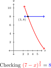
Geometrically, we are looking for where the graph of ![]() intersects the graph of
intersects the graph of ![]() . Below are those graphs and we see the intersection point of both graphs is
. Below are those graphs and we see the intersection point of both graphs is ![]() , thereby checking our solution
, thereby checking our solution ![]() .
.
Example 4.3.1.2
Solve the following equations analytically and verify your answers using a graph.
![]()
Solution:
Solve ![]() for
for ![]() .
.
Proceeding similarly to the above, to solve ![]() , we rewrite
, we rewrite ![]() as
as ![]() and solve:
and solve:
![Rendered by QuickLaTeX.com \[ \begin{array}{rclr} (2t-1)^{\frac{2}{3}} -4 & = & 0 & \\ (\sqrt[3]{2t-1})^2 - 4 & = & 0 & \text{rewrite using Definition 4.3} \\ (\sqrt[3]{2t-1})^2 & = & 4 & \text{isolate the variable term} \\ \sqrt{(\sqrt[3]{2t-1})^2 } & = & \sqrt{4} & \text{extract square roots} \\ |\sqrt[3]{2t-1}| & = & 2 & \sqrt{u^2} = |u| \\ \sqrt[3]{2t-1} & = & \pm 2 & \text{ for } c>0, \, |u| = c \text{ is equivalent to } u = \pm c. \end{array} \]](https://pressbooks.library.tamu.edu/app/uploads/quicklatex/quicklatex.com-ea007c81b35ee51fbb1fa531f19cc698_l3.png)
From ![]() we cube both sides of each equation.
we cube both sides of each equation.
![Rendered by QuickLaTeX.com \[ \begin{array}{rclcrcl} \sqrt[3]{2t-1} & = & -2 & \text{ and } & \sqrt[3]{2t-1} & = & 2 \\ 2t - 1 & = & -8 & \qquad & 2t-1 & = & 8 \\ t & = & - \frac{7}{2} & \qquad & t & = & \frac{9}{2} \end{array} \]](https://pressbooks.library.tamu.edu/app/uploads/quicklatex/quicklatex.com-a5601a35dad2e504f354c62c9e3f22a5_l3.png)
Both of ![]() and
and ![]() are solutions to the given equation.
are solutions to the given equation.
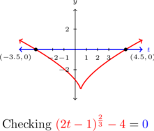
In this case we are looking for where the graph of ![]() intersects the graph of
intersects the graph of ![]() – i.e., the
– i.e., the ![]() -intercepts of the graph of
-intercepts of the graph of ![]() . We find these are
. We find these are ![]() and
and ![]() , as predicted.
, as predicted.
Example 4.3.1.3
Solve the following equations analytically and verify your answers using a graph.
![]()
Solution:
Solve ![]() for
for ![]() .
.
![]() , so we may rewrite
, so we may rewrite ![]() as
as ![]() . Using Definition 4.3, we then have
. Using Definition 4.3, we then have ![]() . One of the square roots is already isolated, thus we can rid ourselves of it by squaring both sides.
. One of the square roots is already isolated, thus we can rid ourselves of it by squaring both sides.
![Rendered by QuickLaTeX.com \[ \begin{array}{rclr} \sqrt{x+3} & = & 2\sqrt{7-x} + 1 & \\ (\sqrt{x+3})^2 & = & (2\sqrt{7-x} + 1)^2 & \text{square both sides} \\ x+3 & = & (2 \sqrt{7-x})^2 + 2 (2 \sqrt{7-x})(1) + 1 & (\sqrt{u})^2 = u \text{ and } (a+b)^2 = a^2 + 2ab +b^2 \\ x+3 & = & 4(7-x) + 4\sqrt{7-x} + 1 & (ab)^2 = a^2b^2 \text{ and, again, } (\sqrt{u})^2 = u \\ x+3 & = & 28-4x+4\sqrt{7-x} + 1 & \\ 5x-26 & = & 4\sqrt{7-x} & \text{isolate } \sqrt{7-x} \\ \end{array} \]](https://pressbooks.library.tamu.edu/app/uploads/quicklatex/quicklatex.com-a769f504dffe97448b8edf362b4a01d5_l3.png)
We square both sides again and get ![]() .
.
![Rendered by QuickLaTeX.com \[ \begin{array}{rclr} 25x^2-260x+676 & = & 16(7-x) & \text{square both sides} \\ 25x^2-244x+564 & =& 0 & \text{set quadratic equal to zero} \\ (x-6)(25x-94) & = & 0 & \text{ factor} \end{array} \]](https://pressbooks.library.tamu.edu/app/uploads/quicklatex/quicklatex.com-c1e2a7203e0ec911b905d94792991d4c_l3.png)
We set each factor equal to zero, using the Zero Product Property to get
![]()
When we go to check these answers, we verify ![]() is a solution, but
is a solution, but ![]() is not. Hence,
is not. Hence, ![]() is an `extraneous’ solution.[1]
is an `extraneous’ solution.[1]
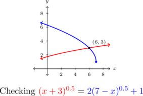
We graph both ![]() and
and ![]() below and confirm there is only one intersection point,
below and confirm there is only one intersection point, ![]() .
.
Example 4.3.1.4
Solve the following equations analytically and verify your answers using a graph.
![]()
Solution:
Solve ![]() for
for ![]() .
.
While we could approach solving ![]() as the previous example, we would encounter cubing binomials[2] which we would prefer to avoid. Instead, we take a step back and notice there are three terms here with the exponent on one term,
as the previous example, we would encounter cubing binomials[2] which we would prefer to avoid. Instead, we take a step back and notice there are three terms here with the exponent on one term, ![]() exactly twice the exponent on another term,
exactly twice the exponent on another term, ![]() . We have ourselves a `quadratic in disguise.’[3]
. We have ourselves a `quadratic in disguise.’[3]
To help us see the forest for the trees, we let ![]() so that
so that ![]() . (Note that root here,
. (Note that root here, ![]() , is odd, so we can use the properties of exponents stated in Theorem 4.3.) Hence,
, is odd, so we can use the properties of exponents stated in Theorem 4.3.) Hence,
![Rendered by QuickLaTeX.com \[ \begin{array}{rclr} 2t^{\frac{2}{3}} + 5t^{\frac{1}{3}} & = & 3 & \text{ in terms of } t \\ 2u^2 + 5u & = & 3 & \text{in terms of } u \\ 2u^2 + 5u - 3 & = & 0 & \\ (2u-1)(u+3) & = & 0 & \text{factoring} \end{array} \]](https://pressbooks.library.tamu.edu/app/uploads/quicklatex/quicklatex.com-e07c781a33212b1a60ed419e0e9cfddc_l3.png)
We set each factor equal to zero, using the Zero Product Property
![Rendered by QuickLaTeX.com \[ \begin{array}{rclcrclr} 2u - 1 & = & 0 & \text{ or } & u+3 & = & 0 & \\[4pt] u & = & \frac{1}{2} & \qquad & u & = & -3 & \\[4pt] t^{\frac{1}{3}} & = & \frac{1}{2} & \text{ or } & t^{\frac{1}{3}} & = & -3 & \text{ replacing } u = t^{\frac{1}{3}} \\[4pt] t & = & \frac{1}{8} & \qquad & t & = & -27 & \text{cube both sides} \end{array} \]](https://pressbooks.library.tamu.edu/app/uploads/quicklatex/quicklatex.com-fac8a4e6c50880d54cba3f8f4e988e36_l3.png)
Both of ![]() and
and ![]() are solutions to our original equation.
are solutions to our original equation.
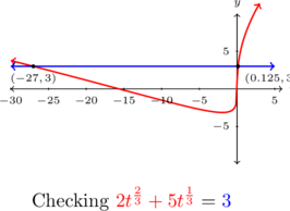
Looking at the graphs of ![]() and
and ![]() , we find two intersection points,
, we find two intersection points, ![]() and
and ![]() as required.
as required.
Example 4.3.1.5
Solve the following equations analytically and verify your answers using a graph.
![]()
Solution:
Solve ![]() for
for ![]() .
.
Next we are to solve ![]() which, when written without negative exponents is:
which, when written without negative exponents is: ![]()
The rational exponents here are ![]() and
and ![]() , both involve an even indexed root (the square root in this case!) which means
, both involve an even indexed root (the square root in this case!) which means ![]()
Moreover, the ![]() resides in the denominator meaning
resides in the denominator meaning ![]() so our equation is really valid only for values of
so our equation is really valid only for values of ![]() where
where ![]() or
or ![]()
Hence, we clear denominators and can apply Theorem 4.3:
![Rendered by QuickLaTeX.com \[ \begin{array}{rclr} \dfrac{2}{(3x-1)^{0.5}} & = & \dfrac{3x}{(3x-1)^{1.5}} & \\ \left[ \dfrac{2}{(3x-1)^{0.5}} \right] \cdot (3x-1)^{1.5} & = & \left[ \dfrac{3x}{(3x-1)^{1.5}} \right ] \cdot (3x-1)^{1.5} & \\ 2 \cdot \dfrac{(3x-1)^{1.5}}{(3x-1)^{0.5}} & = & 3x & \\ 2 (3x-1)^{1.5-0.5} & = & 3x & \text{Theorem 4.3 applies as $3x-1 > 0$.} \\ 2 (3x-1)^{1} & = & 3x & \\ 6x-2 & = & 3x & \\ x & = & \frac{2}{3} & \end{array} \]](https://pressbooks.library.tamu.edu/app/uploads/quicklatex/quicklatex.com-cda4bba16ad2f969dd85f0da5c513942_l3.png)
Because ![]() , we keep it and, sure enough, it is a solution to our original equation.
, we keep it and, sure enough, it is a solution to our original equation.
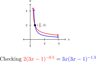
Graphically we see ![]() intersects
intersects ![]() at
at ![]()
Example 4.3.1.6
Solve the following equations analytically and verify your answers using a graph.
![]()
Solution:
Solve ![]() for
for ![]() .
.
Our last equation to solve is ![]() , which, when rewritten without negative exponents is:
, which, when rewritten without negative exponents is: ![]() . Again, the root here (
. Again, the root here (![]() ) is odd, so we can use the exponent properties listed in Theorem 4.3. We begin by clearing denominators:
) is odd, so we can use the exponent properties listed in Theorem 4.3. We begin by clearing denominators:
![Rendered by QuickLaTeX.com \[ \begin{array}{rclr} 6(9-t^2)^{\frac{1}{3}} & = & \frac{4t^2}{(9-t^2)^{\frac{2}{3}}} & \\[10pt] 6(9-t^2)^{\frac{1}{3}} \cdot (9-t^2)^{\frac{2}{3}} & = & \left[ \frac{4t^2}{(9-t^2)^{\frac{2}{3}}} \right ] \cdot (9-t^2)^{\frac{2}{3}} & \\ 6(9-t^2)^{\frac{1}{3} + \frac{2}{3}}& = & 4t^2 & \text{Theorem 4.3 applies because the root here $3$ is odd.} \\ 6(9-t^2)^{1} & = & 4t^2 &\\ 54 - 6t^2 & = & 4t^2 & \\ 10t^2 & = & 54 & \\ t^2 & = & \frac{54}{10} & \\[6pt] t & = & \pm \sqrt{\frac{27}{5}} & \\[6pt] t & = & \pm 3 \sqrt{15}{5} \\[6pt] \end{array} \]](https://pressbooks.library.tamu.edu/app/uploads/quicklatex/quicklatex.com-73206e2e29c52ccd1a1783ef3c0035ff_l3.png)
So ![]() . While not the easiest to check analytically, both of these solutions do work in the original equation.
. While not the easiest to check analytically, both of these solutions do work in the original equation.
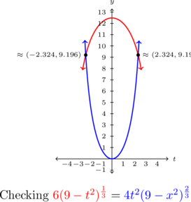
Graphing ![]() and
and ![]() below, we see the graphs intersect when
below, we see the graphs intersect when ![]() .
.
Note that in Example 4.3.1, there are several ways to correctly solve each equation, and we endeavored to demonstrate a variety of methods. For example, for number 1, instead of converting ![]() to a radical equation, we could use Theorem 4.3. The root here (
to a radical equation, we could use Theorem 4.3. The root here (![]() ) is even, thus we know
) is even, thus we know ![]() or
or ![]() . Hence we may apply exponent properties:
. Hence we may apply exponent properties:
![Rendered by QuickLaTeX.com \[ \begin{array}{rclr} (7-x)^{\frac{3}{2}} & = & 8 & \\ \left[(7-x)^{\frac{3}{2}}\right]^{\frac{2}{3}} & = & 8^{\frac{2}{3}} & \text{raise both sides to the $\frac{2}{3}$ power} \\ (7-x)^{\frac{3}{2} \cdot \frac{2}{3}} & = & 4 & \text{Theorem 4.3} \\ (7-x)^{1} & = & 4 \\ \end{array} \]](https://pressbooks.library.tamu.edu/app/uploads/quicklatex/quicklatex.com-61f5158897c4b557afc4abcabe00234a_l3.png)
from which we get ![]() . If we try this same approach to solve number 2, however, we encounter difficulty. From
. If we try this same approach to solve number 2, however, we encounter difficulty. From ![]() , we get
, we get ![]() .
.
![Rendered by QuickLaTeX.com \[ \begin{array}{rclr} (2t-1)^{\frac{2}{3}} & = & 4 & \\ \left[(2t-1)^{\frac{2}{3}} \right]^{\frac{3}{2}} & = & 4^{\frac{3}{2}}& \text{raise both sides to the $\frac{3}{2}$ power} \\ \end{array} \]](https://pressbooks.library.tamu.edu/app/uploads/quicklatex/quicklatex.com-0aeff1081540132679d6d3b28c2dc24f_l3.png)
Given the root here (![]() ) is odd, we have no restriction on
) is odd, we have no restriction on ![]() but the exponent
but the exponent ![]() has an even denominator. Hence, Theorem 4.3 does not apply. That is,
has an even denominator. Hence, Theorem 4.3 does not apply. That is,
![Rendered by QuickLaTeX.com \[ \begin{array}{rcl} \left[(2t-1)^{\frac{2}{3}} \right]^{\frac{3}{2}} & \neq & (2t-1)^{\frac{2}{3} \cdot \frac{3}{2}} \\ & = & (2t-1)^{1} \\ & = & (2t-1) \end{array} \]](https://pressbooks.library.tamu.edu/app/uploads/quicklatex/quicklatex.com-52503bd8b5058d383afd039062ca27a1_l3.png)
Note that if we weren’t careful, we’d have ![]() which gives
which gives ![]() only. We’d have missed the solution
only. We’d have missed the solution ![]() . Truth be told, you can simplify
. Truth be told, you can simplify ![]() – just not using Theorem 4.3. We leave it as an exercise to show
– just not using Theorem 4.3. We leave it as an exercise to show ![]() and, more generally,
and, more generally, ![]() .
.
Our next example is an application of the Cobb Douglas production model of an economy. The Cobb-Douglas model states that the yearly total dollar value of the production output in an economy is a function of two variables: labor (the total number of hours worked in a year) and capital (the total dollar value of the physical goods required for manufacturing.) The equation relating the production output level ![]() , labor
, labor ![]() and capital
and capital ![]() takes the form
takes the form ![]() where
where ![]() ; that is, the production level varies jointly with some power of the labor and capital.
; that is, the production level varies jointly with some power of the labor and capital.
Example 4.3.2
Example 4.3.2.1
In their original paper A Theory of Production[4] Cobb and Douglas modeled the output of the US Economy (using 1899 as a baseline) using the formula
![]()
where ![]() ,
, ![]() , and
, and ![]() were percentages of the 1899 figures for total production, labor, and capital, respectively.
were percentages of the 1899 figures for total production, labor, and capital, respectively.
For 1910, the recorded labor and capital figures for the US Economy are 144% and 208% of the 1899 figures, respectively. Compute ![]() using these figures and interpret your answer.
using these figures and interpret your answer.
Solution:
For 1910, the recorded labor and capital figures for the US Economy are 144% and 208% of the 1899 figures, respectively. Compute ![]() using these figures and interpret your answer.
using these figures and interpret your answer.
In this case,
![Rendered by QuickLaTeX.com \[ \begin{array}{rcl} P & = & 1.01 L^{0.75} K^{0.25} \\ & = & 1.01 (144)^{0.75} (208)^{0.25} \\ & \approx & 159 \end{array} \]](https://pressbooks.library.tamu.edu/app/uploads/quicklatex/quicklatex.com-a86d46ea9c8f3b85ff419ebf14f3bd65_l3.png)
which means the dollar value of the total US Production in 1920 was approximately 159% of what it was in 1899.[5]
Example 4.3.2.2
In their original paper A Theory of Production[6] Cobb and Douglas modeled the output of the US Economy (using 1899 as a baseline) using the formula
![]()
where ![]() ,
, ![]() , and
, and ![]() were percentages of the 1899 figures for total production, labor, and capital, respectively.
were percentages of the 1899 figures for total production, labor, and capital, respectively.
The recorded production value figure for 1920 is 231% of the 1899 figure. Use this to write ![]() as a function of
as a function of ![]() ,
, ![]() . Compute and interpret
. Compute and interpret ![]() .
.
Solution:
The recorded production value figure for 1920 is ![]() of the 1899 figure. Use this to write
of the 1899 figure. Use this to write ![]() as a function of
as a function of ![]() ,
, ![]() . Compute and interpret
. Compute and interpret ![]() .
.
We are given ![]() , so to write
, so to write ![]() as a function of
as a function of ![]() , we need to solve this equation for
, we need to solve this equation for ![]() .
. ![]() and
and ![]() are positive by definition, so we can employ properties of exponents:
are positive by definition, so we can employ properties of exponents:
![Rendered by QuickLaTeX.com \[ \begin{array}{rclr} 231 & = & 1.01 L^{0.75} K^{0.25} & \\[5pt] \dfrac{231}{1.01 L^{0.75}} & = & \dfrac{1.01 L^{0.75} K^{0.25}}{1.01 L^{0.75}} & \text{$L>0$, hence $L^{0.75} \neq 0$.}\\[8pt] K^{0.25} & = & 228.\overline{7128}L^{-0.75} & \text{rewrite} \\[5pt] \left(K^{0.25}\right)^{\frac{1}{0.25}} & = & \left(228.\overline{7128}L^{-0.75}\right)^{\frac{1}{0.25}} & \\[5pt] K^{\frac{0.25}{0.25}} & = & (228.\overline{7128})^{\frac{1}{0.25}} L^{-\frac{0.75}{0.25}} & \text{Theorem 4.3} \\[5pt] K & = & (228.\overline{7128})^{4} L^{-3} & \text{simplify} \\ \end{array} \]](https://pressbooks.library.tamu.edu/app/uploads/quicklatex/quicklatex.com-60355cb15b410179d08c8aee1a0be826_l3.png)
Hence, ![]() where
where ![]() .
.
We find
![]()
meaning that in order to maintain a production level of 231% of 1889 with a labor level at 193% of 1889, the required capital is ![]() that of 1889.[7]
that of 1889.[7]
Example 4.3.2.3
In their original paper A Theory of Production[8] Cobb and Douglas modeled the output of the US Economy (using 1899 as a baseline) using the formula
![]()
where ![]() ,
, ![]() , and
, and ![]() were percentages of the 1899 figures for total production, labor, and capital, respectively.
were percentages of the 1899 figures for total production, labor, and capital, respectively.
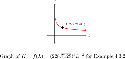
Graph ![]() and interpret the behavior as
and interpret the behavior as ![]() and
and ![]() .
.
Solution:
Graph ![]() and interpret the behavior as
and interpret the behavior as ![]() and
and ![]()
The function ![]() is a Laurent Monomial (see Section 3.2) with
is a Laurent Monomial (see Section 3.2) with ![]() and
and ![]() .
.
As such, as ![]() ,
, ![]() . This means that in order to maintain the given production level, as the available labor diminishes, the capital requirement become unbounded.
. This means that in order to maintain the given production level, as the available labor diminishes, the capital requirement become unbounded.
As ![]() , we have
, we have ![]() meaning that as the available labor increases, the need for capital diminishes.
meaning that as the available labor increases, the need for capital diminishes.
The graph of ![]() is called an `isoquant’ – meaning `same quantity.’ In this context, the graph displays all combinations of labor and capital,
is called an `isoquant’ – meaning `same quantity.’ In this context, the graph displays all combinations of labor and capital, ![]() which result in the same production level, in this case,
which result in the same production level, in this case, ![]() of what was produced in 1889.
of what was produced in 1889.
4.3.1 Section Exercises
In Exercises 1 – 14, solve the equation.


- The Cobb-Douglas production model[9] for the country of Sasquatchia is
 . Here,
  represents the country’s production (measured in thousands of Bigfoot Bullion),
  represents the total labor (measured in thousands of hours) and
  represents the total investment in capital (measured in Bigfoot Bullion.) Let
  and solve for
  as a function of
  . If
. If  , what is
  ? Interpret each of the quantities in this case.
Section 4.3 Exercise Answers can be found in the Appendix … Coming soon
- We invite the reader to see at which point in our machinations
 does check. Knowing a solution is extraneous is one thing; understanding how it came about is another. ↵
 - that is, expanding things like
 . ↵
. ↵ - See Section 0.5.5. ↵
- available here. ↵
- This answer is remarkably accurate. Note: all the dollar values here are recorded in `1880' dollars, per the source article. ↵
- available here. ↵
- The actual recorded figure is 407. ↵
- available here. ↵
- See Example 4.3.2 for more details on these sorts of models. ↵

