7.4 Other Trigonometric Functions

Vanessa Coffelt

7.4 Other Trigonometric Functions

In subsection 7.2.2, we extended the notion of $\sin(\theta)$ and $\cos(\theta)$ from acute angles to any angles using the coordinate values of points on the Unit Circle. In total, there are six circular functions, as listed below.

Definition 7.5 The Circular Functions

Suppose an angle $\theta$ is graphed in standard position.

Let $P(x,y)$ be the point of intersection of the terminal side of $P$ and the Unit Circle.

While we left the history of the name `sine’ as an interesting research project in Section 7.2.2, we take a slight detour here to explain the origin of the names `tangent’ and `secant.’

Consider the acute angle $\theta$ in standard position sketched in the diagram below.

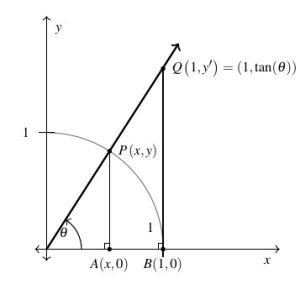
The first quadrant of a cartesian plane. The angle theta is drawn with terminal side in quadrant I. A quarter of the unit circle is included in the graph. A line segment parallel to the y-axis at the point where the terminal side meets the unit circle to the x-axis is labeled with endpoints P(x,y) and A(x,0). A second line parallel to the first line segment has endpoints Q(1,y')=(1,tan(theta)) and B(1,0). — Graphical Representation of Tangent

As usual, $P(x,y)$ denotes the point on the terminal side of $\theta$ which lies on the Unit Circle, but we also consider the point $Q(1,y')$ , the point on the terminal side of $\theta$ which lies on the vertical line $x=1$ .

The word `tangent’ comes from the Latin meaning `to touch,’ and for this reason, the line $x=1$ is called a tangent line to the Unit Circle as it intersects, or `touches’, the circle at only one point, namely $(1,0)$ .

Dropping perpendiculars from $P$ and $Q$ creates a pair of similar triangles $\Delta OPA$ and $\Delta OQB$ . Hence the corresponding sides are proportional. We get $\frac{y'}{y} = \frac{1}{x}$ which gives $y' = \frac{y}{x} = \tan(\theta)$ .

We have just shown that for acute angles $\theta$ , $\tan(\theta)$ is the $y$ -coordinate of the point on the terminal side of $\theta$ which lies on the line $x = 1$ which is tangent to the Unit Circle.

The word `secant’ means `to cut’, so a secant line is any line that `cuts through’ a circle at two points.^[1] The line containing the terminal side of $\theta$ (not just the terminal side itself) is one such secant line as it intersects the Unit Circle in Quadrants I and III.

With the point $P$ lying on the Unit Circle, the length of the hypotenuse of $\Delta OPA$ is $1$ . If we let $h$ denote the length of the hypotenuse of $\Delta OQB$ , we have from similar triangles that $\frac{h}{1} = \frac{1}{x}$ , or $h = \frac{1}{x} = \sec(\theta)$ .

Hence for an acute angle $\theta$ , $\sec(\theta)$ is the length of the line segment which lies on the secant line determined by the terminal side of $\theta$ and `cuts off’ the tangent line $x=1$ .

As we mentioned in Definition 7.3, the `co’ in `cosecant’ and `cotangent’ tie back to the concept of `co’mplementary angles and is explained in detail in Section 8.2.

Not only do these observations help explain the names of these functions, they serve as the basis for a fundamental inequality needed for Calculus which we’ll explore in the Exercises.

In Definition 7.2 we introduced the trigonometric ratios for sine and cosine. There are four more trigonometric ratios which are commonly used and they are defined in the same manner the ratios for sine and cosine are defined using the given right triangle. They are listed below.

Definition 7.6

Suppose $\theta$ is an acute angle residing in the right triangle as depicted below.

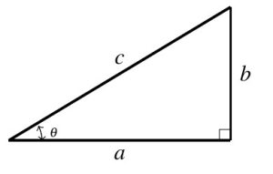
A right triangle with horizontal side, a, vertical side, b, and hypotenuse, c . The angle between sides a and c is labeled theta. The angle between sides c and b is not labeled.. The right angle is between sides a and b. — Right Triangle with angle theta

The tangent of $\theta$ , denoted $\tan(\theta)$ is defined by the ratio: $\tan(\theta) = \dfrac{b}{a}$ , or $\dfrac{\text{`length of opposite'}}{\text{`length of adjacent'}}$ .
The cosecant of $\theta$ , denoted $\csc(\theta)$ is defined by the ratio: $\csc(\theta) = \dfrac{c}{b}$ , or $\dfrac{\text{`length of hypotenuse'}}{\text{`length of opposite'}}$
The secant of $\theta$ , denoted $\sec(\theta)$ is defined by the ratio: $\sec(\theta) = \dfrac{c}{a}$ , or $\dfrac{\text{`length of hypotenuse'}}{\text{`length of adjacent'}}$
The cotangent of $\theta$ , denoted $\cot(\theta)$ is defined by the ratio: $\cot(\theta) = \dfrac{a}{b}$ , or $\dfrac{\text{`length of adjacent'}}{\text{`length of opposite'}}$

We practice these definitions in the following example.

Example 7.4.1

Suppose $\theta$ is an acute angle with $\cot(\theta) = 3$ . Find the values of the remaining five trigonometric ratios: $\sin(\theta)$ , $\cos(\theta)$ , $\tan(\theta)$ , $\csc(\theta)$ , and $\sec(\theta)$ .

Solution:

We are given $\cot(\theta) = 3$ . So, to proceed, we construct a right triangle in which the length of the side adjacent to $\theta$ and the length of the side opposite of $\theta$ has a ratio of $3 = \frac{3}{1}$ . Note there are infinitely many such right triangles – we have produced two below for reference. We will focus our attention on the triangle below on the left and encourage the reader to work through the details using the triangle below on the right to verify the choice of triangle doesn’t matter.

Rendered by QuickLaTeX.com

From the diagram, we see immediately $\tan(\theta) = \frac{1}{3}$ , but in order to determine the remaining four trigonometric ratios, we need to first compute the value of the hypotenuse. The Pythagorean Theorem gives

$\begin{array}{rcl} 1^2 + 3^2 &=& c^2 \\[4pt] c^2 &=& 10 \\[4pt] c &=& \sqrt{10} \end{array}$

Rationalizing denominators, we find

$\sin(\theta) = \frac{1}{\sqrt{10}} = \frac{\sqrt{10}}{10}$

$\cos(\theta) = \frac{3}{\sqrt{10}} = \frac{3\sqrt{10}}{10}$

$\csc(\theta) = \frac{\sqrt{10}}{1} = \sqrt{10}$

$\sec(\theta) = \frac{\sqrt{10}}{3}$

7.4.1 Reciprocal and Quotient Identities

Of the six circular functions, only sine and cosine are defined for all angles $\theta$ . Given $x = \cos(\theta)$ and $y = \sin(\theta)$ in Definition 7.5, it is customary to rephrase the remaining four circular functions in Definition 7.5 in terms of sine and cosine.

Theorem 7.8 Reciprocal and Quotient Identities

$\sec(\theta) = \dfrac{1}{\cos(\theta)}$ , provided $\cos(\theta) \neq 0$ ; if $\cos(\theta) = 0$ , $\sec(\theta)$ is undefined.
$\csc(\theta) = \dfrac{1}{\sin(\theta)}$ , provided $\sin(\theta) \neq 0$ ; if $\sin(\theta) = 0$ , $\csc(\theta)$ is undefined.
$\tan(\theta) = \dfrac{\sin(\theta)}{\cos(\theta)}$ , provided $\cos(\theta) \neq 0$ ; if $\cos(\theta) = 0$ , $\tan(\theta)$ is undefined.
$\cot(\theta) = \dfrac{\cos(\theta)}{\sin(\theta)}$ , provided $\sin(\theta) \neq 0$ ; if $\sin(\theta) = 0$ , $\cot(\theta)$ is undefined.

We call the equations listed in Theorem 7.8 identities because they are relationships which are true regardless of the values of $\theta$ . This is in contrast to conditional equations such as $\sin(\theta) = 1$ which are true for only some values of $\theta$ . We will study identities more extensively in Sections 8.1 and 8.2.

While the Reciprocal and Quotient Identities presented in Theorem 7.8 allow us to always reduce problems involving secant, cosecant, tangent and cotangent to problems involving sine and cosine, it is not always convenient to do so.^[2] It is worth taking the time to memorize the tangent and cotangent values of the common angles summarized below.

Tangent and Cotangent Values of Common Angles

$\begin{array}{|c|c||c|c|} \hline \theta (\text{degrees}) & \theta (\text{radians}) & \tan(\theta) & \cot(\theta) \\ \hline 0^{\circ} & 0 & 0 & \text{undefined} \\ \hline 30^{\circ} & \frac{\pi}{6} & \frac{\sqrt{3}}{3} & \sqrt{3} \\ [2pt] \hline 45^{\circ} & \frac{\pi}{4} & 1 & 1 \\ [2pt] \hline 60^{\circ} & \frac{\pi}{3} & \sqrt{3} & \frac{\sqrt{3}}{3} \\ [2pt] \hline 90^{\circ} & \frac{\pi}{2} & \text{undefined} & 0 \\ [2pt] \hline \end{array}$

Coupling Theorem 7.8 with the Reference Angle Theorem, Theorem 7.2, we get the following.

Theorem 7.9 Generalized Reference Angle Theorem

The values of the circular functions of an angle, if they exist, are the same, up to a sign, of the corresponding circular functions of its reference angle.

More specifically, if $\alpha$ is the reference angle for $\theta$ , then:

$\sin(\theta) = \pm \sin(\alpha), \quad \cos(\theta) = \pm \cos(\alpha) \quad \tan(\theta) = \pm \tan(\alpha)$

and

$\sec(\theta) = \pm \sec(\alpha) \quad \csc(\theta) = \pm \csc(\alpha) \quad \cot(\theta) = \pm \cot(\alpha)$

where the choice of the ( $\pm$ ) depends on the quadrant in which the terminal side of $\theta$ lies.

It is high time for an example.

Example 7.4.2

Example 7.4.2.1a

Compute the exact value of the following, if it exists:

$\sec\left(60^{\circ}\right)$

Solution:

Compute the exact value of $\sec\left(60^{\circ}\right)$ .

According to Theorem 7.8, $\sec\left(60^{\circ}\right) = \frac{1}{\cos\left(60^{\circ}\right)}$ .

Hence, $\sec\left(60^{\circ}\right) = \frac{1}{(1/2)} = 2$ .

Example 7.4.2.1b

Compute the exact value of the following, if it exists:

$\csc\left(\frac{7 \pi}{4} \right)$

Solution:

Compute the exact value of $\csc\left(\frac{7 \pi}{4} \right)$ .

Recall $\sin\left( \frac{7\pi}{4}\right) = - \frac{\sqrt{2}}{2}$ , so

$\begin{array}{rcl} \csc\left( \frac{7\pi}{4}\right) &=& \frac{1}{\sin\left( \frac{7\pi}{4}\right)} \\[4pt] &=& \frac{1}{- \sqrt{2}/2} \\[4pt] &=& - \frac{2}{\sqrt{2}} \\[4pt] &=& - \sqrt{2} \end{array}$

Example 7.4.2.1c

Compute the exact value of the following, if it exists:

$\tan(225^{\circ})$

Solution:

Compute the exact value of $\tan(225^{\circ})$ .

We have two ways to proceed to determine $\tan(225^{\circ})$ . \vskip 0.5em

First, we can use Theorem 7.8 and note that

$\begin{array}{rcl} \tan(225^{\circ}) &=& \frac{\sin(225^{\circ})}{\cos(225^{\circ})} \\[6pt] &=& \frac{\sin(225^{\circ}) }{ \cos(225^{\circ}) } \\[6pt] &=& \frac{-\frac{\sqrt{2}}{2}}{- \frac{\sqrt{2}}{2}} \\[6pt] \tan(225^{\circ}) &=& 1 \end{array}$

Another way to proceed is to note that $225^{\circ}$ has a reference angle of $45^{\circ}$ . Per Theorem 7.9, $\tan(225^{\circ}) = \pm \tan(45^{\circ}) = \pm 1$ .

Because $225^{\circ}$ is a Quadrant III angle, where both the $x$ and $y$ coordinates of points are both negative, and tangent is defined as the ratio of coordinates $\frac{y}{x}$ , we know $\tan(225^{\circ}) > 0$ .

Hence, $\tan(225^{\circ}) = 1$ .

Example 7.4.2.1d

Compute the exact value of the following, if it exists:

$\cot\left(-\frac{7 \pi}{6} \right)$

Solution:

Compute the exact value of $\cot\left(-\frac{7 \pi}{6} \right)$ .

As with the previous example, we have two ways to proceed. Using Theorem 7.8, we have

$\begin{array}{rcl} \cot\left(-\frac{7 \pi}{6} \right) &=& \frac{\cos\left(-\frac{7 \pi}{6} \right)}{\sin\left(-\frac{7 \pi}{6} \right)} \\[6pt] &=& \frac{-\frac{\sqrt{3}}{2}}{\frac{1}{2}} \\[6pt] \cot\left(-\frac{7 \pi}{6} \right) &=& - \sqrt{3} \end{array}$

Alternatively, we note $-\frac{7 \pi}{6}$ is a Quadrant II angle with reference angle $\frac{\pi}{6}$ .

Hence, Theorem7.9 tells us $\cot\left(-\frac{7 \pi}{6} \right) = \pm \cot\left(\frac{\pi}{6} \right) = \pm \sqrt{3}$ . Because $-\frac{7 \pi}{6}$ is a Quadrant II angle, where the $x$ and $y$ coordinates have different signs, and cotangent is defined as the ratio of coordinates $\frac{x}{y}$ , we know $\cot\left(-\frac{7 \pi}{6} \right)<0$ .

Hence, $\cot\left(-\frac{7 \pi}{6} \right) = -\sqrt{3}$ .

Example 7.4.2.2a

Determine all angles which satisfy the given equation.

$\sec(\theta) =2$

Solution:

Determine all angles which satisfy the equation $\sec(\theta) =2$ .

To solve $\sec(\theta) = 2$ , we convert to cosines and get $\frac{1}{\cos(\theta)} = 2$ or $\cos(\theta) = \frac{1}{2}$ .

This is the exact same equation we solved in Example 7.2.4 number 1, so we know the answer is:

$\theta = \frac{\pi}{3} + 2\pi k$ or $\theta = \frac{5\pi}{3} + 2\pi k$ for integers $k$ .

Example 7.4.2.2b

Determine all angles which satisfy the given equation.

$\csc(\theta) = -\sqrt{2}$

Solution:

Determine all angles which satisfy the equation $\csc(\theta) = -\sqrt{2}$ .

To solve $\csc(\theta) = -\sqrt{2}$ , we convert to sines and get $\frac{1}{\sin(\theta)} = - \sqrt{2}$ or $\sin(\theta) = -\frac{\sqrt{2}}{2}$ .

Using the table of values for $\sin(t)$ found below Theorem 7.5 in Section 7.3 we know $\sin \left(\frac{5\pi}{4} \right) = - \frac{\sqrt{2}}{2}$ and $\sin \left(\frac{7\pi}{4} \right) = - \frac{\sqrt{2}}{2}$ .

Thus the answer is: $\theta = \frac{5\pi}{4} + 2\pi k$ or $\theta = \frac{7\pi}{4} + 2\pi k$ for integers $k$ .

Example 7.4.2.2c

Determine all angles which satisfy the given equation.

$\tan(\theta) = \sqrt{3}$

Solution:

Determine all angles which satisfy the equation $\tan(\theta) = \sqrt{3}$ .

From the table of common values, we see $\tan\left(\frac{\pi}{3}\right) = \sqrt{3}$ .

According to Theorem 7.9, we know the solutions to $\tan(\theta) = \sqrt{3}$ must, therefore, have a reference angle of $\frac{\pi}{3}$ .

To find the quadrants in which our solutions lie, we note that tangent is defined as the ratio $\frac{y}{x}$ of points $(x,y)$ on the Unit Circle. Hence, tangent is positive when $x$ and $y$ have the same sign (i.e., when they are both positive or both negative.) This happens in Quadrants I and III.

In Quadrant I, we get the solutions: $\theta = \frac{\pi}{3} + 2\pi k$ for integers $k$ , and for Quadrant III, we get $\theta = \frac{4\pi}{3} + 2\pi k$ for integers $k$ .

While these descriptions of the solutions are correct, they can be combined into one list as $\theta = \frac{\pi}{3} + \pi k$ for integers $k$ .

The latter form of the solution is best understood looking at the geometry of the situation in a diagram.^[3]

Rendered by QuickLaTeX.com

Example 7.4.2.2d

Determine all angles which satisfy the given equation.

$\cot(\theta) = -1$

Solution:

Determine all angles which satisfy the equation $\cot(\theta) = -1$ .

From the table of common values, we see that $\frac{\pi}{4}$ has a cotangent of $1$ , which means the solutions to $\cot(\theta) = -1$ have a reference angle of $\frac{\pi}{4}$ .

To find the quadrants in which our solutions lie, we note that $\cot(\theta) = \frac{x}{y}$ for a point $(x,y)$ on the Unit Circle where $y \neq 0$ . If $\cot(\theta)$ is negative, then $x$ and $y$ must have different signs (i.e., one positive and one negative.)

Hence, our solutions lie in Quadrants II and IV.

Our Quadrant II solution is $\theta = \frac{3\pi}{4} + 2\pi k$ , and for Quadrant IV, we get $\theta = \frac{7\pi}{4} + 2\pi k$ for integers $k$ .

As in the previous problem, we can combine these solutions as: $\theta = \frac{3\pi}{4} + \pi k$ for integers $k$ .

Rendered by QuickLaTeX.com

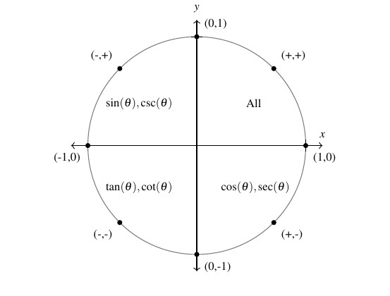
A few remarks about Example 7.4.2 are in order. First note that the signs ( $\pm$ ) of secant and cosecant are the same as the signs of cosine and sine, respectively.

On the other hand, as a result of tangent and cotangent being defined in terms of the ratios of coordinates $x$ and $y$ , tangent and cotangent are positive in Quadrants I and III (where both $x$ and $y$ have the same sign) and negative in Quadrants II and IV (where $x$ and $y$ have opposite signs.)

The diagram below summarizes which circular functions are positive in which quadrants.

A unit circle centered at the origin of the cartesian plane. There are points on the unit circle where the circle meets each axis. There are four additional points marked at the quarter points between the axes, each point includes the signs of x and y in each quadrant. Inside the circle is a list of the trigonometric functions that are positive in that quadrant. The first quadrant says "All", the second quadrant lists sine of theta and cosecant of theta, the third quadrant lists tangent of theta and cotangent of theta, and the fourth quadrant lists cosine of theta and secant of theta. — Positive Circular Functions

Also note it is no coincidence that both of our solutions to the equations involving tangent and cotangent in Example 7.4.2 could be simplified to just one list of angles differing by multiples of $\pi$ .

Indeed, any two angles that are $\pi$ units apart will not only have the same reference angle, but points on their terminal sides on the Unit Circle will be reflections through the origin, as illustrated below.

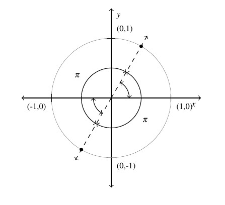
A diagram with two circles, one inside another, centered at the origin of the cartesian plane. The larger circle is a unit circle. The small circle has a radius of less than 1. There is a dashed line from a point on the unit circle in the first quadrant to a point on the unit circle in the third quadrant at an angle pi away from the first point. The angle distance is pi in both directions. — The period of tan (theta) and cot (theta) is pi

It follows that the tangent and cotangent of such angles (if defined) will be the same, which means the period of these function is (at most) $\pi$ .

Using an argument similar to the one we used to establish the period of sine and cosine in Section 7.3, we note that if $\tan(x+p) = \tan(x)$ for all real numbers $x$ , then, in particular, $\tan(p) = \tan(0+p) = \tan(0) = 0$ . Hence, $p$ is a multiple of $\pi$ , and the smallest multiple of $\pi$ is $\pi$ itself.

Hence, the period of tangent (and cotangent) is $\pi$ , and we will see the consequences of this both when solving equations in this section and when graphing these functions in Section 7.5.

As with sine and cosine, the circular functions defined in Definition 7.5 agree with those put forth in Definitions 7.2 and 7.6 in Section 7.2.1 for acute angles situated in right triangles. The argument is identical to the one given in Section 7.2.2 and is left to the reader.

Moreover, Definition 7.5 can be extended to circles of arbitrary radius $r>0$ using the same similarity arguments in Section 7.2.3 to generalize Definition 7.3 to Theorem 7.4 as summarized below.

Theorem 7.10

Suppose $Q(x,y)$ is the point on the terminal side of an angle $\theta$ (plotted in standard position) which lies on the circle of radius $r$ , $x^2+y^2 = r^2$ . Then:

$\sin(\theta) = \dfrac{y}{r} = \dfrac{y}{\sqrt{x^2+y^2}}$
$\cos(\theta)= \dfrac{x}{r} = \dfrac{x}{\sqrt{x^2+y^2}}$
$\tan(\theta) = \dfrac{y}{x}$ , provided $x \neq 0$
$\sec(\theta) = \dfrac{r}{x} = \dfrac{\sqrt{x^2+y^2}}{x}$ , provided $x \neq 0$
$\csc(\theta) = \dfrac{r}{y} = \dfrac{\sqrt{x^2+y^2}}{y}$ , provided $y \neq 0$
$\cot(\theta) = \dfrac{x}{y}$ , provided $y \neq 0$

We make good use of Theorem 7.10 in the following example.

Example 7.4.3

Example 7.4.3.1

Use Theorem 7.10 to solve the following.

Suppose the terminal side of $\theta$ , when plotted in standard position, contains the point $Q(3,4)$ . Calculate the values of the six circular functions of $\theta$ .

Solution:

Suppose the terminal side of $\theta$ , when plotted in standard position, contains the point $Q(3,4)$ . Calculate the values of the six circular functions of $\theta$ .

Given $x = 3$ and $y=4$ and $x^2+y^2 = r^2$ , then $(3)^2+(4)^2 = r^2$ so $r^2 = 25$ , or $r = 5$ . Theorem 7.10 tells us

$\begin{array}{rcl} \sin(\theta) &=& \frac{4}{5} \\[4pt]\cos(\theta) &=& \frac{3}{5} \\[4pt] \tan(\theta) &=& \frac{4}{3}\\[4pt] \sec(\theta) &=& \frac{5}{3} \\[4pt] \csc(\theta) &= & \frac{5}{4} \\[4pt] \cot(\theta) &=& \frac{3}{4} \end{array}$

Rendered by QuickLaTeX.com

Example 7.4.3.2

Use Theorem 7.10 to solve the following.

Suppose $\theta$ is a Quadrant IV angle with $\cot(\theta) = -4$ . Calculate the values of the five remaining circular functions of $\theta$ .

Solution:

Suppose $\theta$ is a Quadrant IV angle with $\cot(\theta) = -4$ . Calculate the values of the five remaining circular functions of $\theta$ .

In order to use Theorem 7.10, we need to find a point $Q(x,y)$ which lies on the terminal side of $\theta$ , when $\theta$ is plotted in standard position.

We have that $\cot(\theta) = -4 = \frac{x}{y}$ . $\theta$ is a Quadrant IV angle, so we also know $x>0$ and $y< 0$ . Rewriting $-4 = \frac{4}{-1}$ , we choose^[4] $x = 4$ and $y = -1$ so that $r = \sqrt{x^2+y^2} = \sqrt{(4)^2 + (-1)^2} = \sqrt{17}$ .

Applying Theorem 7.10, we find

$\begin{array}{rcl} \sin(\theta) &=& - \frac{1}{\sqrt{17}} = -\frac{\sqrt{17}}{17} \\[4pt] \cos(\theta) &=& \frac{4}{\sqrt{17}} = \frac{4 \sqrt{17}}{17} \\[4pt] \tan(\theta) &=& -\frac{1}{4} \\[4pt] \sec(\theta) &=& \frac{\sqrt{17}}{4} \\[4pt] \csc(\theta) &=& - \sqrt{17} \end{array}$

Rendered by QuickLaTeX.com

Example 7.4.3.3

Compute $\sin\left(\theta\right)$ , where $\sec(\theta) = -\sqrt{5}$ and $\theta$ is a Quadrant II angle.

Solution:

Compute $\sin\left(\theta\right)$ , where $\sec(\theta) = -\sqrt{5}$ and $\theta$ is a Quadrant II angle.

To find $\sin(\theta)$ using Theorem 7.10, we need to determine the $y$ -coordinate of a point $Q(x,y)$ on the terminal side of $\theta$ , when $\theta$ is plotted in standard position, and the corresponding radius $r$ .

Given $\sec(\theta) = \frac{r}{x}$ and $r > 0$ , we rewrite $\sec(\theta) = \frac{r}{x} = -\sqrt{5} = \frac{\sqrt{5}}{-1}$ and take $r = \sqrt{5}$ and $x = -1$ .

To find $y$ , we substitute $x=-1$ and $r=\sqrt{5}$ into $x^2+y^2 = r^2$ to get $(-1)^2+y^2=(\sqrt{5})^2$ . We find $y^2 = 4$ or $y = \pm 2$ . We were told $\theta$ is a Quadrant II angle, thus we select $y = 2$ .

Hence, $\sin(\theta) = \frac{y}{r} = \frac{2}{\sqrt{5}} = \frac{2 \sqrt{5}}{5}$ .

Rendered by QuickLaTeX.com

Example 7.4.3.4

Compute $\cos\left(\theta\right)$ , where $\tan(\theta) = 3$ and $\pi < \theta < \frac{3\pi}{2}$ .

Solution:

Compute $\cos\left(\theta\right)$ , where $\tan(\theta) = 3$ and $\pi < \theta < \frac{3\pi}{2}$ .

We are told $\tan(\theta) = 3$ and $\pi < \theta < \frac{3\pi}{2}$ , so we know $\theta$ is a Quadrant III angle.

To find $\cos(\theta)$ using Theorem 7.10, we need to find the $x$ -coordinate of a point $Q(x,y)$ on the terminal side of $\theta$ , when $\theta$ is plotted in standard position, and the corresponding radius, $r$ .

Given $\tan(\theta) = \frac{y}{x}$ and $\theta$ is a Quadrant III angle, we rewrite $\tan(\theta) = 3 = \frac{-3}{-1} = \frac{y}{x}$ and choose $x = -1$ and $y = -3$ . From $x^2+y^2 = r^2$ , we get $r = \sqrt{10}$ .

Hence, $\cos(\theta) = \frac{x}{r} = \frac{-1}{\sqrt{10}} = -\frac{\sqrt{10}}{10}$ .

Rendered by QuickLaTeX.com

As we did in Section 7.2.3, we may consider $\tan(t)$ , $\sec(t)$ , $\csc(t)$ , and $\cot(t)$ as functions of real numbers by associating each real number $t$ with an angle $\theta$ measuring $t$ radians as discussed in Section 7.2 and using Definition 7.5, or, more generally, Theorem 7.10.

Alternatively, we could define each of these four functions in terms of $f(t) = \sin(t)$ and $g(t) = \cos(t)$ as demonstrated in Theorem 7.8. For example, we could simply define $\sec(t) = \frac{1}{\cos(t)}$ , so long as $\cos(t) \neq 0$ .

Either way, we have the means to explore these functions in greater detail. Before doing so, we’ll need practice with these additional four circular functions courtesy of the Exercises.

We are overdue for an example.

Example 7.4.4

Example 7.4.4.1

The angle of inclination from a point on the ground 30 feet away to the top of Lakeland’s Armington Clocktower^[5] is $60^{\circ}$ . Determine the height of the Clocktower to the nearest foot.

Solution:

The angle of inclination from a point on the ground 30 feet away to the top of Lakeland’s Armington Clocktower. Determine the height of the Clocktower to the nearest foot.

We can represent the problem situation using a right triangle as shown below on the left.

If we let $h$ denote the height of the tower, then we have $\tan\left(60^{\circ}\right) = \frac{h}{30}$ . From this we get an exact answer of $h = 30 \tan\left(60^{\circ}\right) = 30 \sqrt{3}$ feet.

Using a calculator, we get the approximation $51.96$ which, when rounded to the nearest foot, gives us our answer of $52$ feet.

Rendered by QuickLaTeX.com

Example 7.4.4.2

The Americans with Disabilities Act (ADA) stipulates the incline on an accessibility ramp be $5^{\circ}$ . If a ramp is to be built so that it replaces stairs that measure 21 inches tall, how long does the ramp need to be? Round your answer to the nearest inch.

Solution:

The Americans with Disabilities Act (ADA) stipulates the incline on an accessibility ramp be $5^{\circ}$ . If a ramp is to be built so that it replaces stairs that measure 21 inches tall, how long does the ramp need to be? Round your answer to the nearest inch.

We diagram the situation below using $\ell$ to represent the unknown length of the ramp.

We have $\sin\left(5^{\circ} \right)= \frac{21}{\ell}$ so that $\ell = \frac{21}{\sin\left(5^{\circ} \right)} \approx 240.95$ inches.

Hence, the ramp is $241$ inches long.

Rendered by QuickLaTeX.com

Example 7.4.4.3

In order to determine the height of a California Redwood tree, two sightings from the ground, one 200 feet directly behind the other, are made. If the angles of inclination were $45^{\circ}$ and $30^{\circ}$ , respectively, how tall is the tree to the nearest foot?

Solution:

In order to determine the height of a California Redwood tree, two sightings from the ground, one 200 feet directly behind the other, are made. If the angles of inclination were $45^{\circ}$ and $30^{\circ}$ , respectively, how tall is the tree to the nearest foot?

Sketching the problem situation, we find ourselves with two unknowns: the height $h$ of the tree and the distance $x$ from the base of the tree to the first observation point.

Rendered by QuickLaTeX.com

Luckily, we have two right triangles to help us find each unknown, as shown below. From the triangle below on the left, we get $\tan\left(45^{\circ}\right) = \frac{h}{x}$ . From the triangle below on the right, we see $\tan\left(30^{\circ}\right) = \frac{h}{x+200}$ .

Rendered by QuickLaTeX.com

As $\tan\left(45^{\circ}\right) = 1$ , the first equation gives $\frac{h}{x} = 1$ , or $x = h$ . Substituting this into the second equation gives $\frac{h}{h+200} = \tan\left(30^{\circ}\right) = \frac{\sqrt{3}}{3}$ . Clearing fractions, we get $3h = (h+200) \sqrt{3}$ . The result is a linear equation for $h$ , so we expand the right hand side and gather all the terms involving $h$ to one side.

$\begin{array}{rcl} 3h & = & (h+200)\sqrt{3} \\ [5pt] 3h & = & h \sqrt{3} + 200 \sqrt{3} \\ [5pt] 3h - h \sqrt{3} & = & 200 \sqrt{3} \\ [5pt] (3-\sqrt{3}) h & = & 200 \sqrt{3} \\ [5pt] h & = & \dfrac{200\sqrt{3}}{3-\sqrt{3}} \approx 273.20 \\ \end{array}$

Hence, the tree is approximately $273$ feet tall.

7.4.2 Section Exercises

In Exercises 1 – 15, $\theta$ is an acute angle. Use the given trigonometric ratio to find the exact values of the remaining trigonometric ratios of $\theta$ .

$\sin(\theta) = \dfrac{3}{5}$
$\tan(\theta) = \dfrac{12}{5}$
$\csc(\theta) = \dfrac{25}{24}$
$\sec(\theta) = 7$
$\csc(\theta) = \dfrac{10\sqrt{91}}{91}$
$\cot(\theta) = 23$
$\tan(\theta) = 2$
$\sec(\theta) = 4$
$\cot(\theta) = \sqrt{5}$
$\cos(\theta) = \dfrac{1}{3}$
$\cot(\theta) = 2$
$\csc(\theta) = 5$
$\tan(\theta) = \sqrt{10}$
$\sec(\theta) = 2\sqrt{5}$
$\cos(\theta) = 0.4$
A tree standing vertically on level ground casts a 120 foot long shadow. The angle of elevation from the end of the shadow to the top of the tree is $21.4^{\circ}$ . Find the height of the tree to the nearest foot.
The broadcast tower for radio station WSAZ (Home of “Algebra in the Morning with Carl and Jeff”) has two enormous flashing red lights on it: one at the very top and one a few feet below the top. From a point 5000 feet away from the base of the tower on level ground the angle of elevation to the top light is $7.970^{\circ}$ and to the second light is $7.125^{\circ}$ . Find the distance between the lights to the nearest foot.
In Section 7.2.2 we defined the angle of inclination (also known as the angle of elevation) and in this exercise we introduce a related angle – the angle of depression (also known as the angle of declination). The angle of depression of an object refers to the angle whose initial side is a horizontal line above the object and whose terminal side is the line-of-sight to the object below the horizontal. This is represented schematically below.
1. Show that if the horizontal is above and parallel to level ground then the angle of depression (from observer to object) and the angle of inclination (from object to observer) will be congruent because they are alternate interior angles.
2. From a firetower 200 feet above level ground in the Sasquatch National Forest, a ranger spots a fire off in the distance. The angle of depression to the fire is $2.5^{\circ}$ . How far away from the base of the tower is the fire?
3. The ranger in part 18b sees a Sasquatch running directly from the fire towards the firetower. The ranger takes two sightings. At the first sighting, the angle of depression from the tower to the Sasquatch is $6^{\circ}$ . The second sighting, taken just 10 seconds later, gives the the angle of depression as $6.5^{\circ}$ . How far did the Saquatch travel in those 10 seconds? Round your answer to the nearest foot. How fast is it running in miles per hour? Round your answer to the nearest mile per hour. If the Sasquatch keeps up this pace, how long will it take for the Sasquatch to reach the firetower from his location at the second sighting? Round your answer to the nearest minute.
When I stand 30 feet away from a tree at home, the angle of elevation to the top of the tree is $50^{\circ}$ and the angle of depression to the base of the tree is $10^{\circ}$ . What is the height of the tree? Round your answer to the nearest foot.
From the observation deck of the lighthouse at Sasquatch Point 50 feet above the surface of Lake Ippizuti, a lifeguard spots a boat out on the lake sailing directly toward the lighthouse. The first sighting had an angle of depression of $8.2^{\circ}$ and the second sighting had an angle of depression of $25.9^{\circ}$ . How far had the boat traveled between the sightings?
A guy wire 1000 feet long is attached to the top of a tower. When pulled taut it makes a $43^{\circ}$ angle with the ground. How tall is the tower? How far away from the base of the tower does the wire hit the ground?

In Exercises 22 – 41, compute the exact value or state that it is undefined.

$\tan \left( \dfrac{\pi}{4} \right)$
$\sec \left( \dfrac{\pi}{6} \right)$
$\csc \left( \dfrac{5\pi}{6} \right)$
$\cot \left( \dfrac{4\pi}{3} \right)$
$\tan \left( -\dfrac{11\pi}{6} \right)$
$\sec \left( -\dfrac{3\pi}{2} \right)$
$\csc \left( -\dfrac{\pi}{3} \right)$
$\cot \left( \dfrac{13\pi}{2} \right)$
$\tan \left( 117\pi \right)$
$\sec \left( -\dfrac{5\pi}{3} \right)$
$\csc \left( 3\pi \right)$
$\cot \left( -5\pi \right)$
$\tan \left( \dfrac{31\pi}{2} \right)$
$\sec \left( \dfrac{\pi}{4} \right)$
$\csc \left( -\dfrac{7\pi}{4} \right)$
$\cot \left( \dfrac{7\pi}{6} \right)$
$\tan \left( \dfrac{2\pi}{3} \right)$
$\sec \left( -7\pi \right)$
$\csc \left( \dfrac{\pi}{2} \right)$
$\cot \left( \dfrac{3\pi}{4} \right)$

In Exercises 42 – 45, use the given the information to determine the quadrant in which the terminal side of the angle lies when plotted in standard position.

$\sin(\theta) > 0$ but $\tan(\theta) < 0$
$\cot(\alpha) > 0$ but $\cos(\alpha) < 0$
$\sin(\beta) > 0$ and $\tan(\beta) > 0$
$\cos(\gamma) > 0$ but $\cot(\gamma) < 0$

In Exercises 46 – 59, use the given the information to compute the exact values of the circular functions of $\theta$ .

$\sin(\theta) = \dfrac{3}{5}$ with $\theta$ in Quadrant II
$\tan(\theta) = \dfrac{12}{5}$ with $\theta$ in Quadrant III
$\csc(\theta) = \dfrac{25}{24}$ with $\theta$ in Quadrant I
$\sec(\theta) = 7$ with $\theta$ in Quadrant IV
$\csc(\theta) = -\dfrac{10\sqrt{91}}{91}$ with $\theta$ in Quadrant III
$\cot(\theta) = -23$ with $\theta$ in Quadrant II
$\tan(\theta) = -2$ with $\theta$ in Quadrant IV
$\sec(\theta) = -4$ with $\theta$ in Quadrant II
$\cot(\theta) = \sqrt{5}$ with $\theta$ in Quadrant III
$\cos(\theta) = \dfrac{1}{3}$ with $\theta$ in Quadrant I
$\cot(\theta) = 2$ with $0 < \theta < \dfrac{\pi}{2}$
$\csc(\theta) = 5$ with $\dfrac{\pi}{2} < \theta < \pi$
$\tan(\theta) = \sqrt{10}$ with $\pi < \theta < \dfrac{3\pi}{2}$
$\sec(\theta) = 2\sqrt{5}$ with $\dfrac{3\pi}{2} < \theta < 2\pi$

In Exercises 60 – 67, use your calculator to approximate the given value to three decimal places. Make sure your calculator is in the proper angle measurement mode!

$\csc(78.95^{\circ})$
$\tan(-2.01)$
$\cot(392.994)$
$\sec(207^{\circ})$
$\csc(5.902)$
$\tan(39.672^{\circ})$
$\cot(3^{\circ})$
$\sec(0.45)$

In Exercises 68 – 82, find all of the angles which satisfy the equation.

$\tan(\theta) = \sqrt{3}$
$\sec(\theta) = 2$
$\csc(\theta) = -1$
$\cot(\theta) = \dfrac{\sqrt{3}}{3}$
$\tan(\theta) = 0$
$\sec(\theta) = 1$
$\csc(\theta) = 2$
$\cot(\theta) = 0$
$\tan(\theta) = -1$
$\sec(\theta) = 0$
$\csc(\theta) = -\dfrac{1}{2}$
$\sec(\theta) = -1$
$\tan(\theta) = -\sqrt{3}$
$\csc(\theta) = -2$
$\cot(\theta) = -1$

In Exercises 83 – 90, solve the equation for $t$ . Give exact values.

$\cot(t) = 1$
$\tan(t) = \dfrac{\sqrt{3}}{3}$
$\sec(t) = -\dfrac{2\sqrt{3}}{3}$
$\csc(t) = 0$
$\cot(t) = -\sqrt{3}$
$\tan(t) = -\dfrac{\sqrt{3}}{3}$
$\sec(t) = \dfrac{2\sqrt{3}}{3}$
$\csc(t) = \dfrac{2\sqrt{3}}{3}$

In Exercises 91 – 98, write the given function as a nontrivial decomposition of functions as directed.

For $f(t) = 3t^2 + 2 \tan(3t)$ , find functions $g$ and $h$ so that $f=g+h$ .
For $f(\theta) = \sec(\theta) - \tan(\theta)$ , find functions $g$ and $h$ so that $f=g-h$ .
For $f(t) = -\csc(t) \cot(t)$ , find functions $g$ and $h$ so that $f=gh$ .
For $r(t) = \dfrac{\tan(3t)}{t}$ , find functions $f$ and $g$ so $r = \dfrac{f}{g}$ .
For $T(\theta) =\tan(4 \theta)$ , find functions $f$ and $g$ so $T = g \circ f$ .
For $s(\theta) = \sec^{2}(\theta)$ , find functions $f$ and $g$ so $s = g \circ f$ .
For $L(x) = \ln (\sin(x) )$ , find functions $f$ and $g$ so $L = g \circ f$ .
For $\ell(\theta) = \ln | \sec(\theta) - \tan(\theta)|$ , find find functions $f$ , $g$ , and $h$ so $\ell = h \circ (f-g)$ .
Let $S(t) = \sin(t)$ and $C(t) = \cos(t)$ , $F(t) = \tan(t)$ , and $G(t) = \cot(t)$ . Explain why $F = \dfrac{S}{C}$ but $F \neq \dfrac{1}{G}$ . HINT: Think about domains $\ldots$
For each function $T(t)$ listed below, compute the average rate of change over the indicated interval.^[6] What trends do you notice? Compare your answer with what you discovered in Section 7.2.2 number 65. Be sure your calculator is in radian mode!
$\begin{array}{|r||c|c|c|} \hline T(t) & [-0.1, 0.1] & [-0.01, 0.01] &[-0.001, 0.001] \\ \hline \tan(t) &&& \\ \hline \tan(2t) &&& \\ \hline \tan(3t) &&& \\ \hline \tan(4t) &&& \\ \hline \end{array}$
We wish to establish the inequality for Use the diagram from the beginning of the section, partially reproduced below, to answer the following.
1. Show that triangle $OPB$ has area $\frac{1}{2} \sin(\theta)$ and triangle $OQB$ has area $\frac{1}{2} \tan(\theta)$ .
2. Show that the circular sector $OPB$ with central angle $\theta$ has area $\frac{1}{2} \theta$ .
3. Comparing areas, show that $\sin(\theta) < \theta < \tan(\theta)$ for $0 < \theta < \frac{\pi}{2}.$
4. Use the inequality $\sin(\theta) < \theta$ to show that $\frac{\sin(\theta)}{\theta} < 1$ for $0 < \theta < \frac{\pi}{2}.$
5. Use the inequality $\theta < \tan(\theta)$ to show that $\cos(\theta) < \frac{\sin(\theta)}{\theta}$ for $0 < \theta < \frac{\pi}{2}.$ Combine this with the previous part to complete the proof.
Show that $\cos(\theta) < \frac{\sin(\theta)}{\theta} < 1$ also holds for $-\frac{\pi}{2}< \theta < 0$ .

Compare this with the definition given in Section 1.3.4. ↵
As we shall see shortly, when solving equations involving secant and cosecant, we usually convert back to cosines and sines. However, when solving for tangent or cotangent, we usually stick with what we're dealt. ↵
See Example 7.2.4 number 3 in Section 7.2.2 for another example of this kind of simplification of the solution. ↵
We could have just as easily chosen $x=8$ and $y=-2$ - just so long as $x>0$ , $y<0$ and $\frac{x}{y} = -4$ . ↵
Named in honor of Raymond Q. Armington, Lakeland's Clocktower has been a part of campus since 1972. ↵
See Definition1.11 in Section 1.3.4 for a review of this concept, as needed. ↵